The hardware design is actually started with a BOM. In the early design, the initial
estimation system must obtain a preliminary BOM LIST, get the cost information by the BOM,
and quote according the cost information.
After start the project , the BOM is the main work point of the begining period. when you
modify or upgrade or rework, you have to spend a lot of time on the BOM.
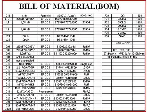
BOM forms are different from different companies, but there are a few key elements need to
mention:
Necessary information:
Component Numbering,Component Mark,Components Description,Components Package,Component
Company,Component Manufacture Part Number,Component Quantity.
The BOM generated by the software contains only the component number, component
description, and company component number. And each item is discrete. If there are 15
resistors of 2K OHM, 0603, 1%, then there are 15 rows. We need to do a lot of work to merge
the same items.
The above work, if you use the your eyes to do it, i think it need take a few days at
least, and may with many errors. Then,how to do this job more quickly and correct?
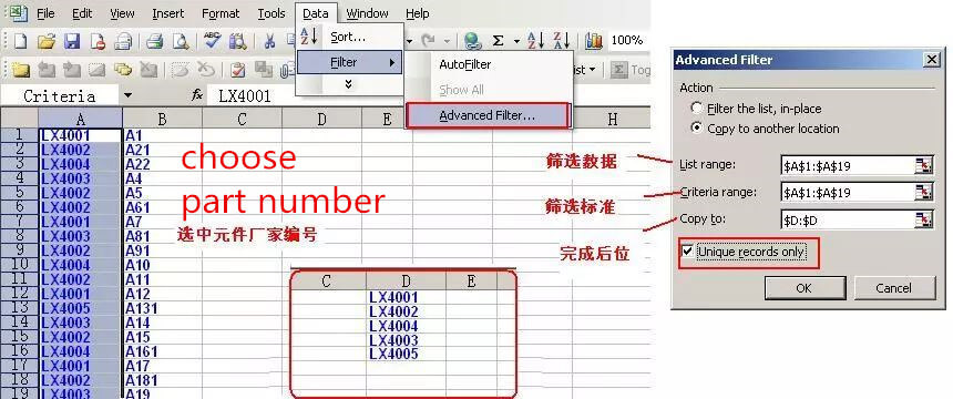
1. First Step:use the Advanced Filter of Data of Excel
2.Second Step:Use formula: COUNTIF(range,criteria),Range is the Cell Area which the number
of cells meet your requirement,Criteria determines which cells will be counted, in the form
of numbers, expressions or text.
3.Third Step: Use Logical judgment formula:=IF(A3=H3,CONCATENATE(C2,”,”,B3),C2) to get the
Combination Mark Number.
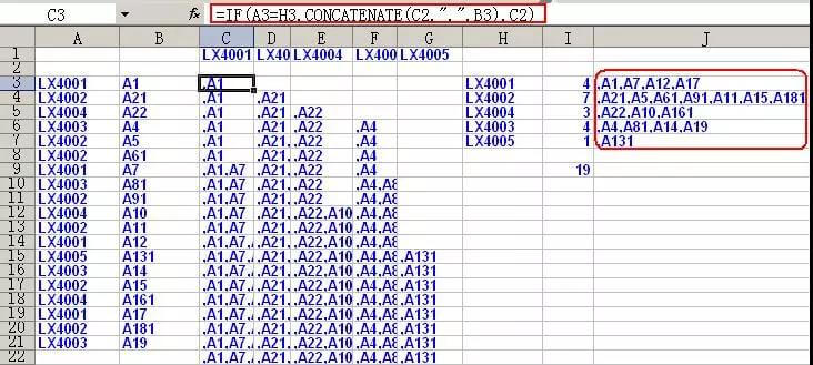
The CONCATENATE means Combine several text items into one text
item,the formula:CONCATENATE(text1,text2……)
In the following section, we take resistance as an example to check the mark and package
and organization, accuracy and voltage. First make a table that describing the device.
Can get accuracy, package and voltage by Composite function:
=INDEX(C:C,MATCH(CONCATENATE(LEFT(I3,5),RIGHT(I3,1)),B:B,0))
=INDEX(C:C,MATCH(MID(I3,6,2),B:B,0))
LEFT function: LEFT (text, num_chars) The Text is the text string containing the characters
to be extracted. Num_chars specifies the number of characters to be extracted by LEFT.
MID function: MID (text, start_num, num_chars) the Text is a text string containing
characters to be extracted. Start_num is the position of the first character to be
extracted in the text.
RIGHT function: RIGHT(text, num_chars) The Text is the text string containing the
characters to be extracted. Num_chars specifies the number of characters that you want
RIGHT to extract.
The MATCH function has two functions, both of which return a position. One is to determine
the exact location of a value in a region in a column. Another one is to determine the
location of a given value in the sorted list, which does not require an exact match. The
formula is: MATCH (lookup_value, lookup_array, match_type) lookup_value is the value to be
searched. Lookup_array: The area to look for (must be a row or a column).
Match_type: Matching form, with 0, 1, and -1 three options: “0” means an accurate search.
“1” means that the search is less than or equal to the maximum value of the check value,
and the search area must be in ascending order. “-1” means that the search is greater than
or equal to the minimum value of the search value, and the search area must be sorted in
descending order. The above search, if there is no matching value, returns #N/A.
The function INDEX() takes two forms: an array and a quote. Array forms usually return a
numeric or numeric array; the quote form usually returns quote.
INDEX(array,row_num,column_num) Returns the value of the specified cell or array of cells
in the array.
Array is a cell range or array constant
Row_num is the row number of a row in the array from which the function returns a value.
Column_num is the column series number of a column in the array from which the function
returns a value. Note that Row_num and column_num must point to a cell in array, otherwise
the function INDEX returns error value the #REF!
Through the above EXCEL tricks, we can BOM List more quickly and correctly.